Brian Jing
11/19/23
BackgroundIn my previous blog (The Data Science Workflow), I explained the three steps required for every data science project: setting up the project, data analysis, and model building. However, since data science teams can extend to over 20 people, not everyone works on each step together; people typically specialize in one aspect of the project, as people typically do for any project in every company. Today, I will focus on the model-building aspect of the data science workflow by explaining common data modeling techniques, with more examples using R in RStudio.
RegressionTo start off, regression models in data science are techniques to determine the strengths of explanatory variables in determining the response.
Linear regressionIs the most common. This modeling technique can be thought of as a linear equation, creating a line of best fit for all instances of the data to represent the relationships between the explanatory variable(s) and the response variable, as visualized below.
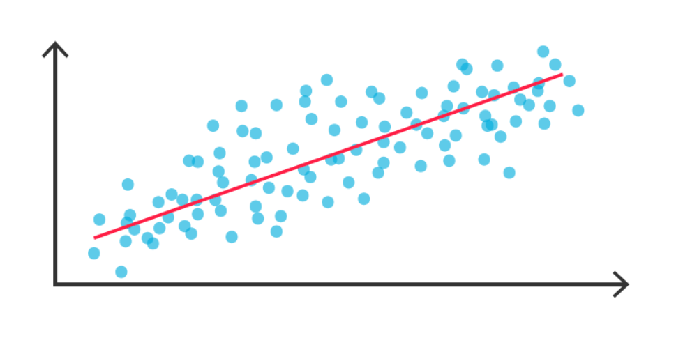
Graphical Representation of Linear Regression
In regression models, there can also be multiple explanatory variables, but there can only be one response variable, unless advanced modeling techniques are used, but those will be covered in later blogs. You can think of the linear equation as “y = a + b1x1 + b2x2 + … + bnxn”, with y as the response variable, every x-value as the amount of each explanatory variable, n as the number of explanatory variables, each b-value as the weight of each explanatory variable in determining the response variable, and the a value as the value of the response variable without any explanatory variables.
This graph above, though, is just a way of abstracting, or simplifying the logic behind a linear regression model. In reality, linear regression models return a variety of numeric values.
To perform linear regression in R, you can either use the lm() function or glm() function, both of which are built into R. lm(), which stands for linear model, represents a simple linear regression model, which mostly deals with the aforementioned “linear equation”-type regression, and glm(), which stands for generalized linear model, being able to represent more general types of regression models, such as with graphical representations that are nonlinear.
The lm() function can be implemented like this in R:
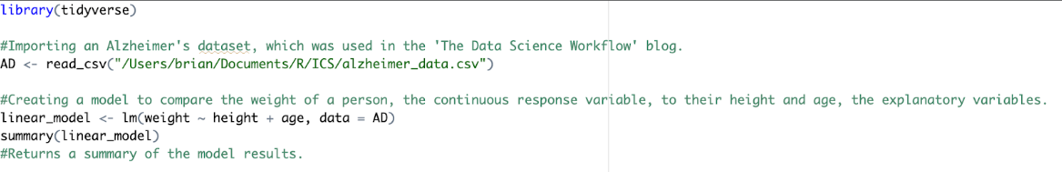
The lm() constructor takes in two required arguments: the formula comparing the explanatory variable(s) (right of ~) and the response variable (left of ~), separated with a squiggly returns as follows:
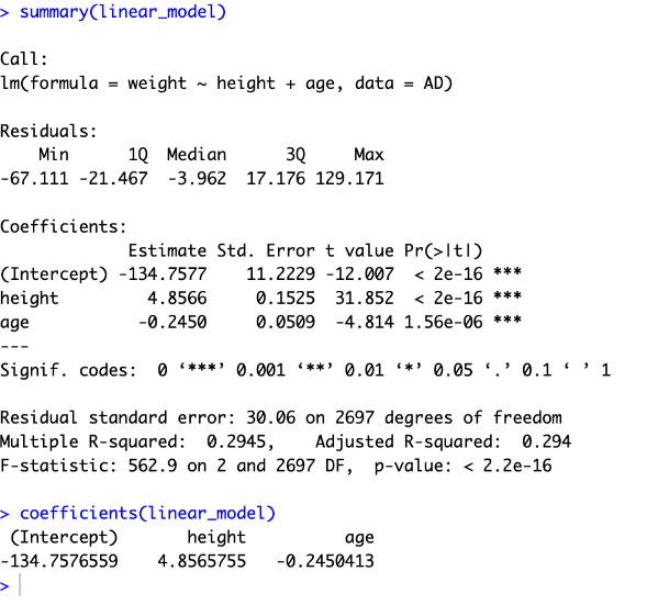
While this may seem like a lot to digest, it is the job of the data scientist to know which values they must use and interpret those values for their project. The most commonly analyzed is the area in the middle:
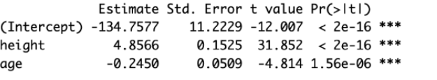
The “estimate” value under (Intercept) represents the a-value in the aforementioned linear regression equation,
meaning that the average weight , and the estimates for height and age represent the b-value coefficients of those explanatory variables,
or the change that an increase by one in those variables would have in the response variable. For instance,
ne year of an increase in age will decrease a person’s weight by 0.245 pounds.
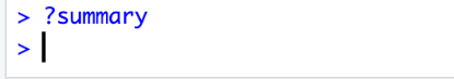
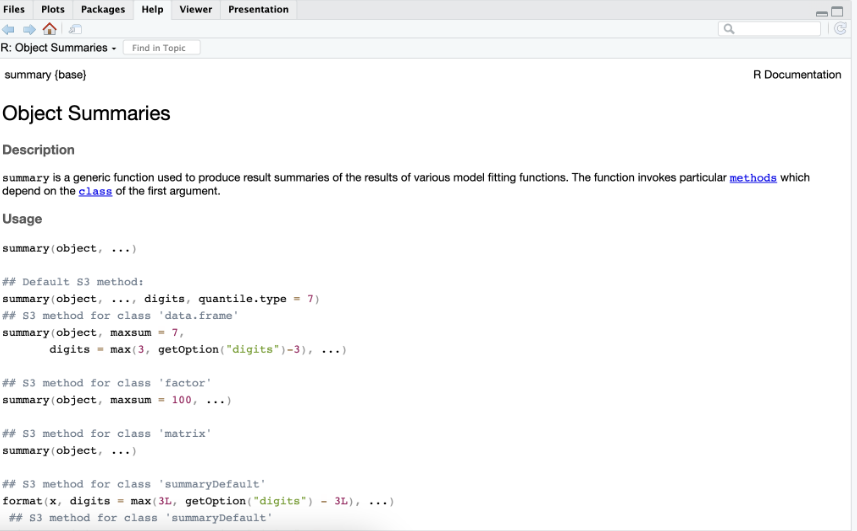
The other values have separate uses, but they would be used much less frequently, and it would be too much to cover in a singular blog. If you are curious, however, you can type “?summary” in the terminal, which will return a description of the values the summary function returns in the bottom right box in RStudio. You can type “?[functionname]” in the terminal for any R function, which will return a description in the same place.
There are other functions that can be performed to display different model results as well, such as coefficients(modelname) or print(modelname), but these will return results that are simply just smaller parts of what is returned by summary().
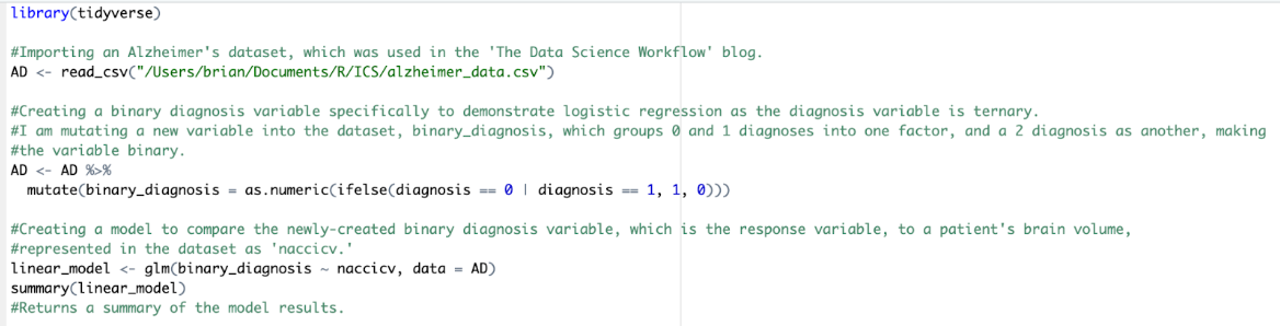
glm() can deal with various types of regression, but another common type of regression it can model is logistic regression, which deals with binary response variables, as opposed to linear regression, which typically deals with continuous response variables. An example of that should look as follows:
is the same thing as logistic regression, but this time dealing with response variables that are non-continuous but more than just binary (ex: ternary, quaternary, etc.). Implementation works as follows:
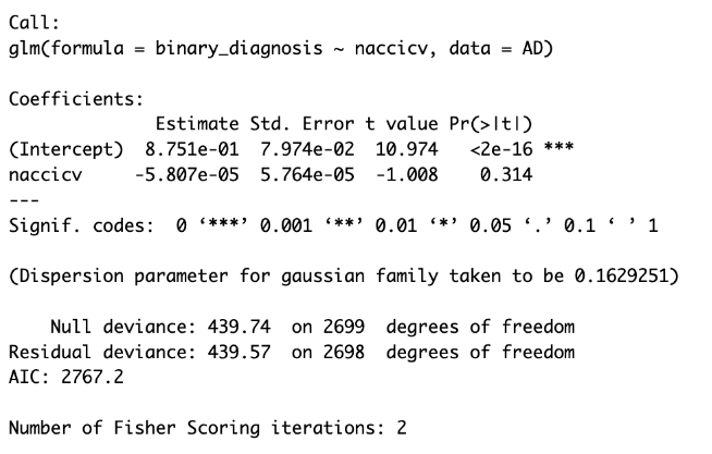
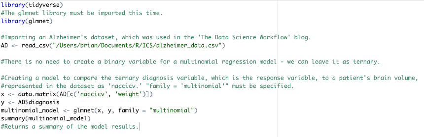
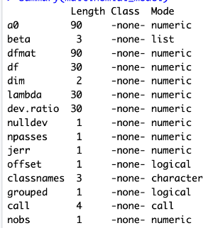
Again, choosing which values to interpret varies by your goal, but the most important are the a0 and beta values, which represent the a and b coefficients for the explanatory and response variables.
More advanced regression techniques include LASSO regression, which eliminates certain explanatory variables based on importance, and ANOVA regression, but as those are not so common, they will not be covered in this blog.
Another prominent modeling technique is classification, which deals with classifying data points into categories based on their features. An example using the Alzheimer’s dataset would be grouping people into different diagnoses based on their brain anatomy, and this could be used in conjunction with regression modeling, as that will identify the most important variables needed to determine a diagnosis, making classification easier.
K-Nearest NeighborsIs one of these types of models that is easy to visualize. This modeling technique classifies a certain attribute of a data point by looking at it’s K, or the number of, nearest neighbors on a graph. This k-value can be set to whatever is desired, but the optimal value varies case by case, and the nearest neighbors are essentially the data points that are closest in terms of the values that you would like to compare the data points by in order to classify them. In the example below, a data point is being classified as blue due to the different categories of data points around it, as the majority of the 5 nearest neighbors on the graph are blue.
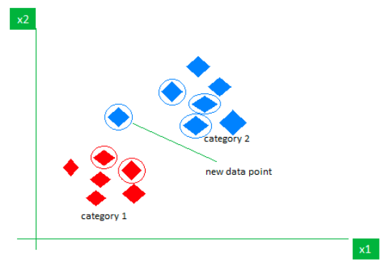
Graphical Representation of the K-Nearest Neighbors Algorithm
Here’s how the implementation of this would look in R, using the Alzheimer’s dataset:
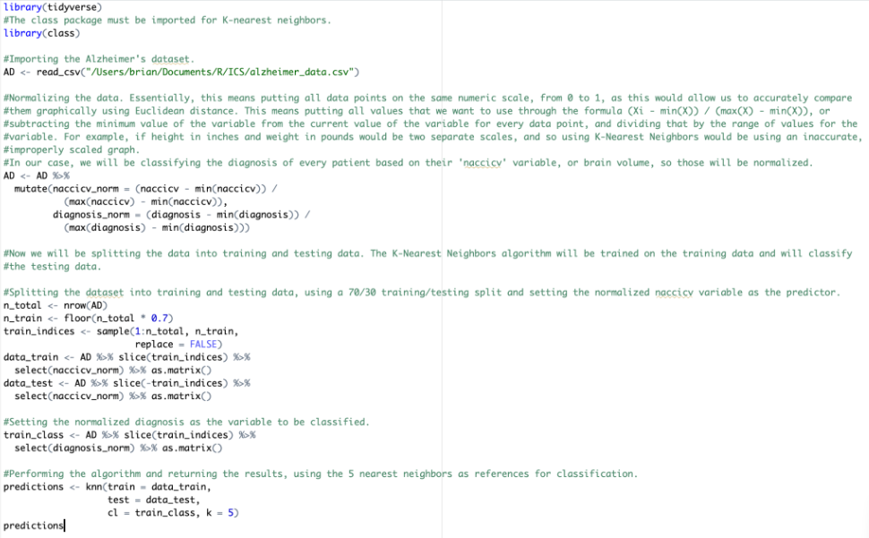
This will return a diagnosis classification for every patient:
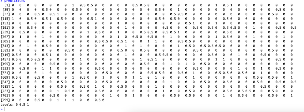
The diagnosis variable is still normalized, as it is only on a scale of 0 to 1, but it still shows the distinct (no to mild to severe Alzheimer’s) diagnoses. This will be the same for any numeric variable, but the classifications should be distinct and recognizable enough in most cases to make conclusions about the data. Furthermore, the denormalization process is much more complex. There is also a way to use K-Nearest Neighbors clustering to classify variables that are not numeric, but that also involves complex manipulations that will not be covered in this blog.
Another classification model is the randomForest model, aptly named so because of its use of decision trees in classifying variables. Each decision tree is a graph shaped in a tree form, starting from the top with a question and guiding the variable down through a series of questions until it reaches a classification. In the example below, the car variable is taken through a series of yes or no questions to eventually be classified as “buy” or “don’t buy.”
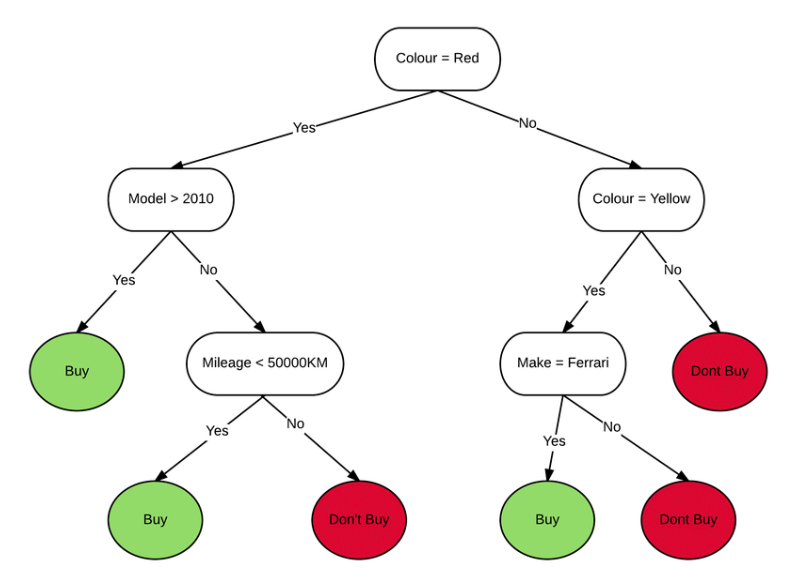
Example of a Decision Tree
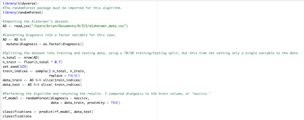
However, the accuracies of these individual decision trees are very low as they are heavily generalized. So, a randomForest model combines multiple, sometimes up to thousands, of these decision trees in order to eventually display an accurate classification of every instance of a variable in R. Implementation is as follows:
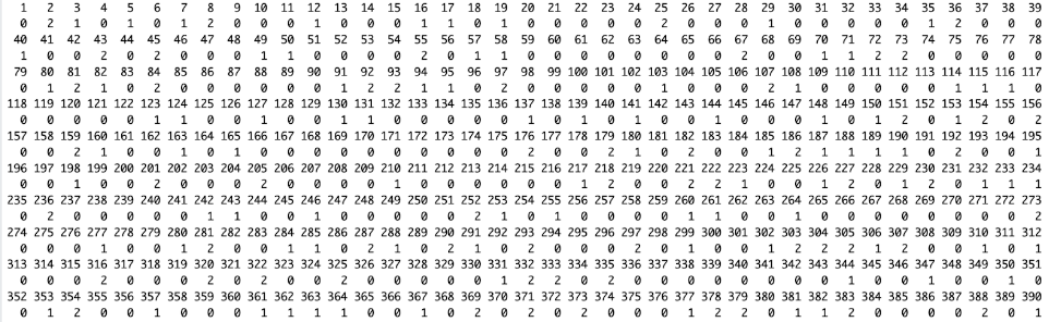
This should classify every patient as a distinct diagnosis, this time in the original scale of 0, 1, and 2.
While there are many more common classification modeling techniques, the K-Nearest Neighbors and randomForest models are two of the most widely used.
Final ThoughtWhile regression and classification models are extremely common in data science, many more exist and serve different functions. Knowing these two broad modeling techniques, however, are useful for starting your data science journey, and can be applied to various types of projects. Some modeling techniques not mentioned in this blog will be useful in specific instances as well, such as clustering, but ultimately, as you pursue more data science projects, you will become more familiar with diverse modeling techniques while researching and experimenting with them.
If you would like datasets to create your own data science projects on, however, they can be found online. A popular website is kaggle.com, and datasets can be found in the “Datasets” page on the left.

From here, you can download any dataset you find interesting, and you can even post your data science projects in the “Code” section, also found on the left of the website.
Overall, I hope this blog has given you an idea of where to start when building data science models, and that it inspires you to pursue your own data science project. In the next blog, I will be taking a step back to the prerequisite of data science projects: having data. I will be focusing on data collection techniques as well as preprocessing data in R before starting data science projects to make sure the data is accurate and optimized.