Brian Jing
8/6/23
Regarded as the “sexiest job of the 21st century,” data science is one of the fastest-growing career paths and branches of computer science; its guarantee of a six-figure salary alongside its vitality for companies’ growth makes it an incredibly appealing field.1 Typically, data scientists make important decisions and manage products for businesses through a combination of computing and statistical methods.
Because of its relevance to the job market, I am writing this article about the process used in data science to make these decisions, often dubbed the “data science workflow,”2 in order to provide you readers with exposure to the procedures taking place behind the scenes of the rapidly-growing field. Throughout this article, I will be using R, a commonly used programming language in data science, to demonstrate this workflow.
All data science projects differ in some sense, but generally, the data science workflow follows an extensive four-step process:
Setting the FrameworkBefore starting your data science project, you need to set it up. In this case, since I am using R, I will start by downloading RStudio, a popular environment for R programming, through this link: https://posit.co/download/rstudio-desktop/.
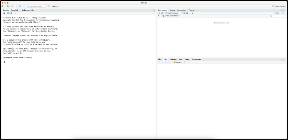
Once RStudio is downloaded and opened, it should look like this:
The next step is to set the context for the project. You must develop a specific research question intended to produce a conclusion about, obviously, data, which you must also either collect or have ready. I will be using an example Alzheimer’s dataset to demonstrate this step, with the meaning of every variable defined in this spreadsheet. Each row in this file contains a patient, and every column is a different attribute of the patient, such as their Alzheimer’s diagnosis, age, and more. My research question will be: “How does brain size affect Alzheimer’s diagnosis?”.
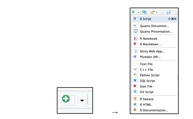
To create a new R file, you need to click the green “plus” button on the top left corner, and create a new “R Script” file.
You should get a blank screen, where you can then type in your code. For now, press ctrl+s to save, move, and name the file as you desire. Make sure the file ends in “.R”.
The next step in answering your research question is exploratory data analysis; also called “data wrangling,” EDA is a way of analyzing your data to find trends and patterns. Since datasets are often too large to naively search through every combination of variables, the research question should be used to narrow down which variables you want to study and find relationships between. Through EDA, you need to find trends to determine which variables will be used as explanatory (independent) and response (dependent) variables in your final model.
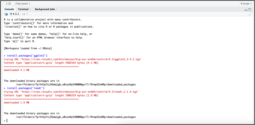
Most of the time, this is done by visualizing the data with graphs. In R specifically, a common way of doing this would be with the “ggplot2” package.3 To use this package, install the package in the console at the bottom left of RStudio. The “readr” package should also be installed in order to read the data from your dataset and use it in your graph. It should all look like this once you’re done:
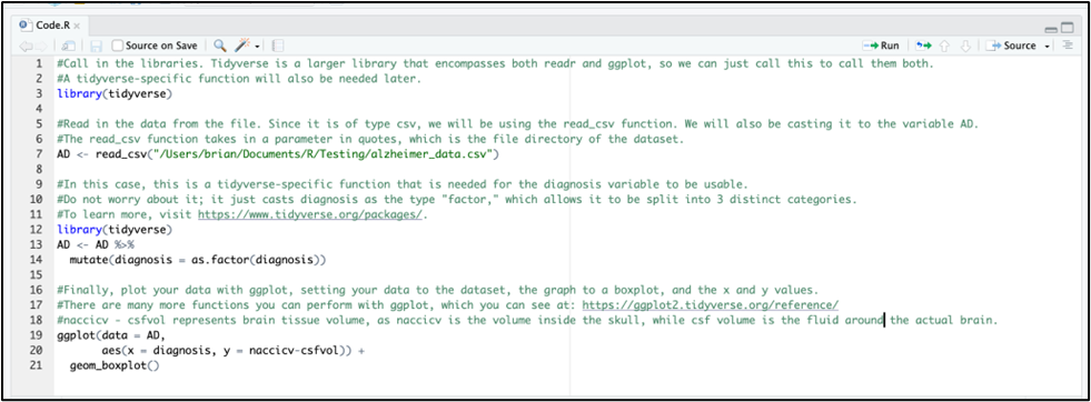
To create a ggplot to perform EDA, you must first read in the data with the “readr” package, and then input that data into the ggplot constructor. It should look like this:
To run code, you must highlight all the lines that you want to run, and then either press the “Run” button at the top right of the code panel, or press ctrl+enter. A quick way to run everything on the file would be to press ctrl+a (to highlight everything) and then ctrl+enter to run it. You should get a graph like this in “plots” on the bottom right:
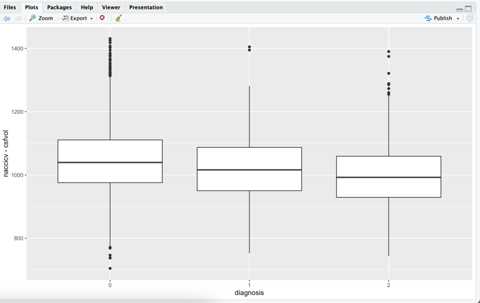
Once you perform EDA enough, you should find trends between certain variables that answer your question. For instance, since my question is how brain size affects diagnosis and my graph shows that it decreases as Alzheimer’s diagnosis goes up, I can conclude that Alzheimer’s decreases brain volume. From here I can move onto building my final model with these variables.
Build A ModelThe final step in your project should be the model. It should dive deeper into the relationships between variables that you found through EDA. Different types of models serve different functions, but the most common type of model is a regression model, which aims to precisely estimate the relationship between explanatory and response variables. The two most common regression models are simple linear and logistic regression models. Typically, linear regression is used with nonbinary response variables, while logistic regression deals with binary response variables (yes/no, 0/1).
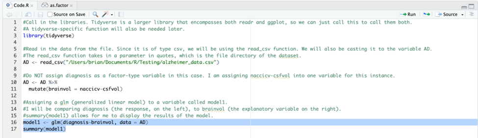
Since my response variable is Alzheimer’s diagnosis, with stages 0, 1, and 2, I will be using linear regression for my model. The code for the model will be shown here:
The summary() function should return the following in the console:
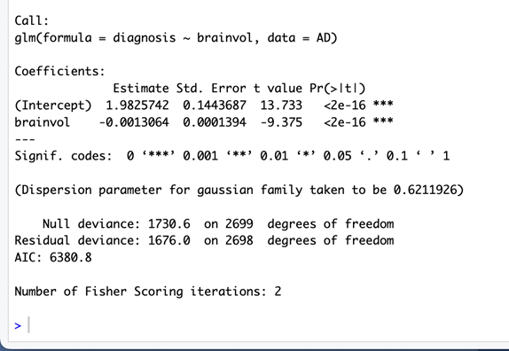
However, just returning these values is not enough; a skilled data scientist should be able to make sense of what they want to extract from the data and present. In my case, I will be using the “Estimate” value. In short, it is the weight of that variable’s impact on the response variable. Since it is a negative value, it means that it has an inverse relationship with Alzheimer’s diagnosis, which checks out when compared to the graph. However, it does not seem to have a big impact on it, since its weight is only ~0.001. This weight is usually relative, but in our case it is still very small.
Making these findings requires knowledge about the meanings of the different values that are returned, which you must find out separately for every different research question. Also, you should always test different types of models and their accuracies, which I will go into more detail about in the next blog.
In the end, your findings should be presented to an audience to spread the information and to make sure it is accurate. In data science, every problem is a story as you are making new insights based on data, and so you must present it as one by presenting the first three steps of the data science workflow in a chronological, engaging manner. Also be sure to explain your findings in a way that allows for the general public to understand, making sure to define any data science jargon that you use in your presentation.
Whether it be to predict the weather or to find patterns within a deadly disease, the data science workflow should always be followed in data science projects. I hope that you readers will someday make impactful data science models with this workflow if you ever choose to pursue a data science career.