Brian Jing
02/16/24
IntroductionBefore I start this blog, I want to establish how it will be structured. This blog is a crash course of the NumPy (“Numerical Python”) Python package, which contains a multitude of functions for mathematical computing that are useful in data science. Though I’ve used R for all my other blogs, I will switch to Python from now on due to its greater versatility and wider use throughout data science. Throughout this blog, I will use the Housing Price Prediction Dataset, provided by Kaggle user Muhammad Bin Imran, to demonstrate NumPy’s usability in working with datasets. The follow-along code for this blog is linked here - have it open while you read for a better learning experience.
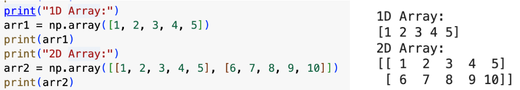
NumPy Arrays: An OverviewNumPy revolves around working with arrays - array objects in NumPy are of the type ndarray, on which you can perform many versatile, efficient NumPy functions. Here are the most basic that you should know for data science projects: np.array() creates an ndarray, with however many dimensions you want. arrayname.ndim gives the number of dimensions in the ndarray.
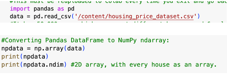
When used in conjunction with the pandas library (used to read files), you can also perform these functions on already-created CSV files. np.array(dataname) converts a Pandas DataFrame into a NumPy ndarray.
To access different elements within an array, you would use array[index you want to access]. With multiple-dimension arrays, you would use multiple index parameters. (ex: for 2d array, you would say array[index of array, index of element within array]. For an index, you can use x:y, where it accesses multiple indices from x to y, not including y. Just putting “:” makes it so that all elements are included. Using this to slice through multiple indices is called slicing. Here it is in action:
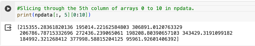
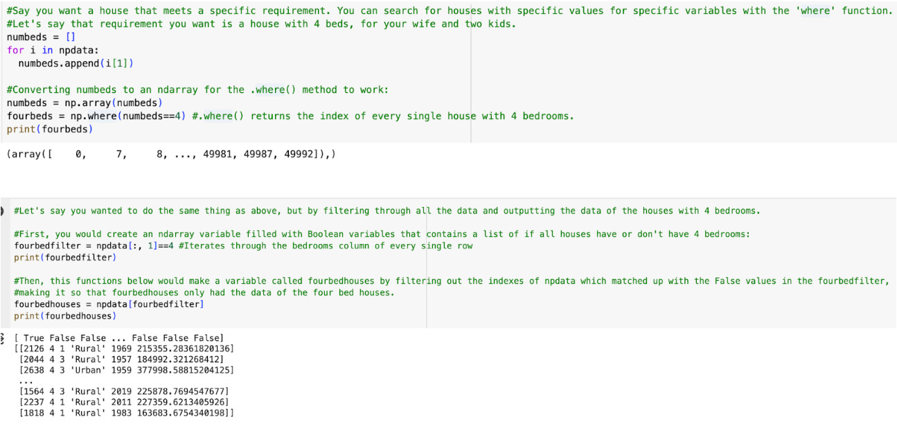
means all arrays in the 2-D array, and parameter 5 means the 4th element in each array. Array iterating, searching, and filtering also comes in handy when you want to look at only certain parts of your data:
ufuncs (Universal Functions) in NumPy are functions for ndarrays which allow for vectorization (operating on the vector/array as a whole rather than having to iterate over it). This allows for increased efficiency and speed.
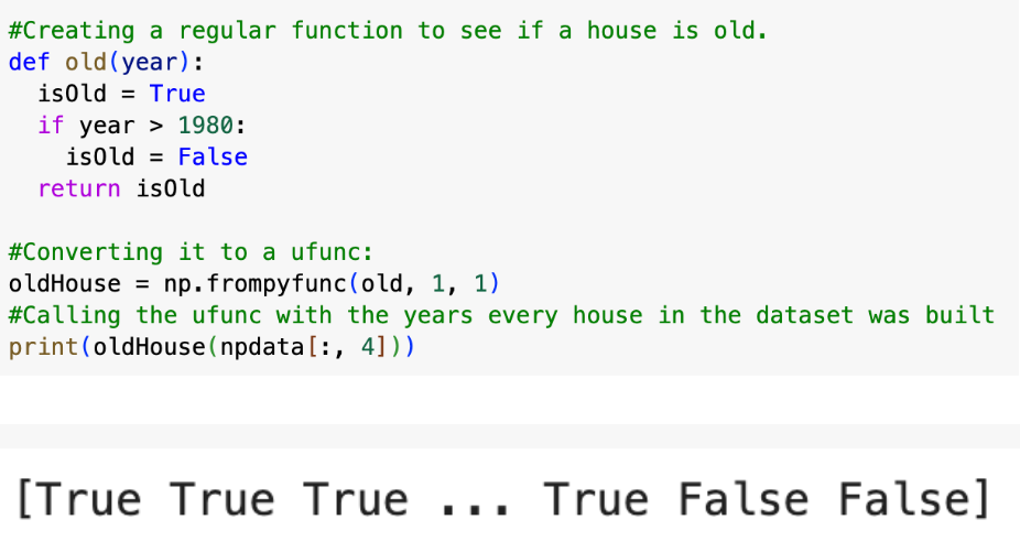
To create your own ufunc, you must first create a regular Python function with def(). Then, you must convert it to a ufunc with the NumPy function frompyfunc(function, inputs, outputs). The three parameters listed are the name of the regular function, the number of inputs in the ufunc, and the number of outputs in the ufunc. Both the inputs and outputs are ndarrays. Here’s an example with the houses dataset:
There are predefined ufuncs in NumPy. Simple arithmetics ufuncs are the most commonly used. There are a multitude of arithmetic operations that can be used for vector arithmetic, from add() and subtract() all the way to trigonometry and set operations, which take ndarrays as arguments. However, listing all of those ufuncs would cause this blog to become unreasonably long, so I won’t, especially since they aren’t too useful for the houses dataset. If you would like to research those arithmetic ufuncs, I will link a W3Schools tutorial here. To see all the operations on this tutorial, scroll down the left-hand column menu below the heading “NumPy ufunc”.
The final important aspect of NumPy I will cover is its numpy.random module, which allows for random data distributions to be created. It supports a wide variety of statistical distributions, from binomial to Pareto to Rayleigh. These randomly-created distributions allow for simulation, or taking random samples of data to test or train models. In this blog, I will only show the process of creating and visualizing daa distributions.
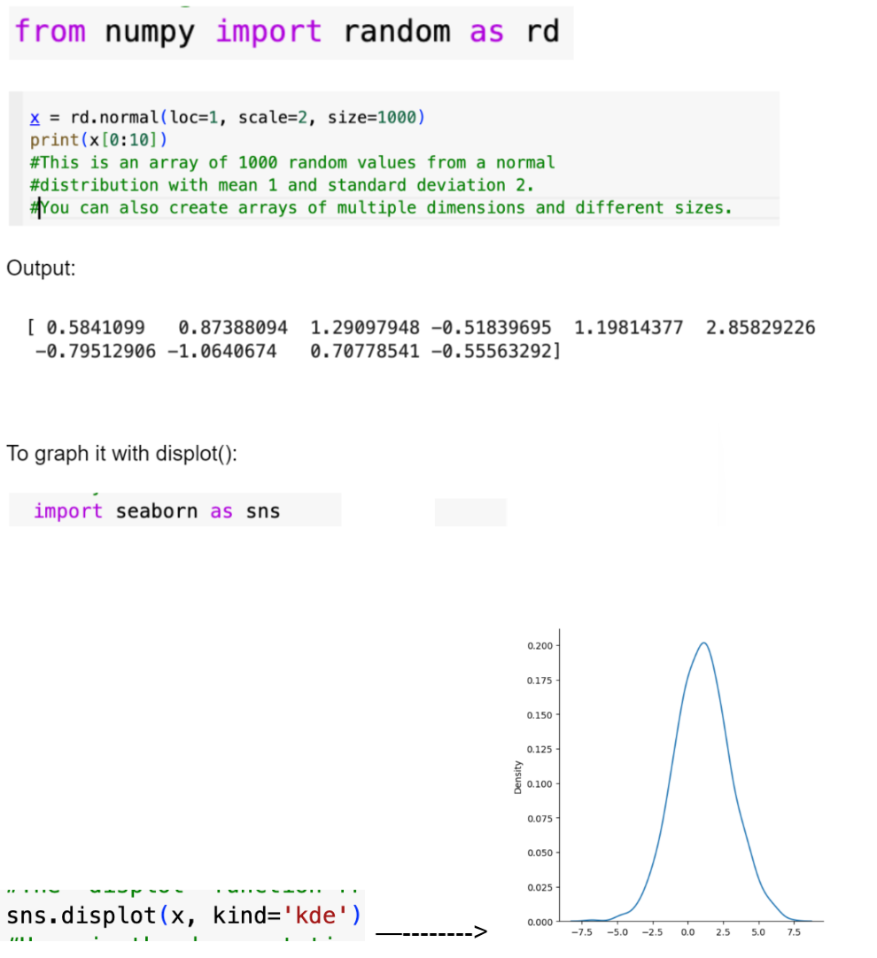
In this blog I will be covering four essential data distributions for data science: normal, uniform, multinomial, and chi square distributions. You can view more data distributions on the W3Schools page under “NumPy Random.” They will be used alongside the Seaborn package, specifically the displot function, which allows for visualization of these data distributions.
To import numpy.random, type from numpy import random.
1. Normal DistributionsThree parameters: loc (mean/where is the peak of bell), scale (standard deviation), size (shape of returned array) How to create one with NumPy:
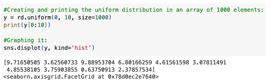
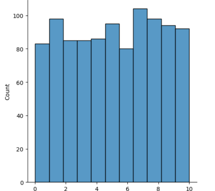
Three parameters, a (lower bound), b(upper bound), size (of returned array) To create and graph a uniform distribution with NumPy.
Basically, creating every data distribution is just:
random.distributionname(parameters).
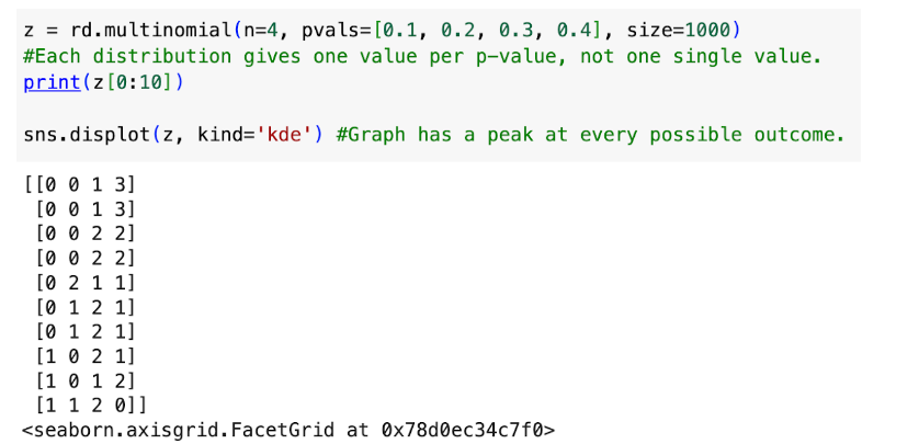
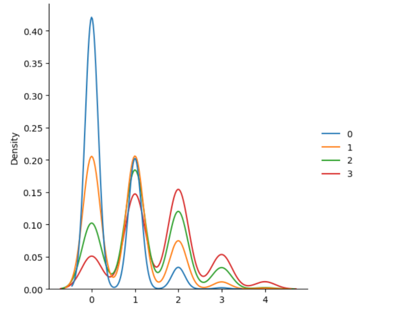
Three parameters: n(num of possible outcomes), pvals (probability of every outcome, must be given as a list with size n), size (of returned array)
To create and graph:
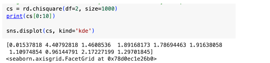
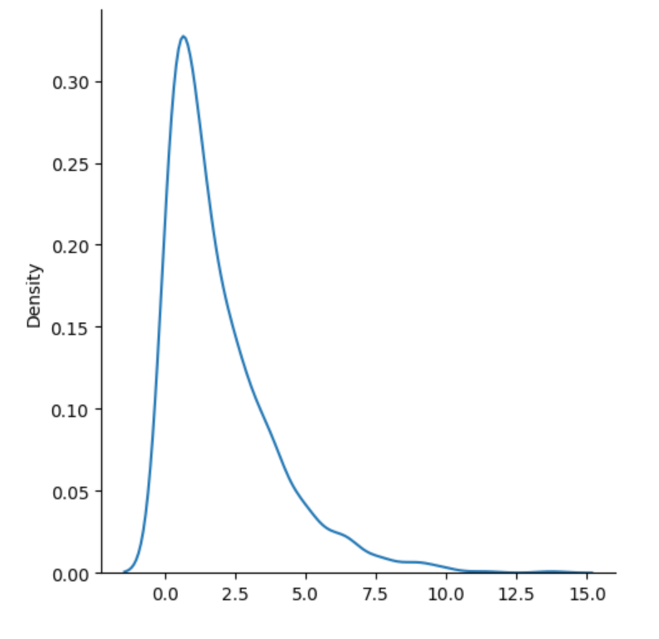
The chi square distribution compares the squared differences between observed and expected values (chi-square statistic) with the probability of each value. Two parameters: df (degrees of freedom), size (of returned array) Degrees of freedom basically means however many independent variables there are.
Most data distributions require lots of statistical knowledge to understand and use. Unlike distributions 1-3, the chi square distribution, like most, isn’t straightforward to understand. As a data scientist, you must put time into having a statistical understanding of your data and the different types of data distributions and models
To create and graph:
This was a very basic overview of NumPy, which is commonly used throughout data science projects in all parts of the data science workflow. I hope you learned from this blog, and I hope that this blog interested you enough about NumPy to go and research more about it yourself. When looking to expand your data science knowledge further, make sure to look for even more advanced packages and modules, and also more advanced functions within NumPy that I didn’t cover myself. Again, if you missed it, here is the link to the follow-along code for this blog, and here is the link to the more in-depth NumPy tutorial on W3Schools that you can use for your own further research.
As a final note, thank you for reading my blog! I hope it helped you on your journey as a data scientist.